PID Control: The Algorithm That Runs the World

If there’s one algorithm that every roboticist needs to understand, it’s the PID controller. PID stands for Proportional-Integral-Derivative, and it’s the feedback control algorithm that runs thermostats, motor speed controllers, drone stabilizers, industrial processes, and countless other systems.

The Problem PID Solves

Imagine you want a motor to spin at exactly 100 RPM. You apply some voltage, but the motor spins at 85 RPM — it’s 15 RPM short of your target. How much do you increase the voltage?

The naive answer is “increase it until you hit 100 RPM.” But if you increase it too much, the motor overshoots to 120 RPM. Then you reduce it, and it drops to 90 RPM. You end up oscillating forever.

PID solves this by computing a correction based on three terms. All three live inside a feedback loop: you compare where you are against where you want to be, react to that error, and measure the result — over and over.

The Three Terms

Proportional (P): correction proportional to the current error.

• Error = Setpoint − Current Value
• P output = Kp × Error
• Large error → large correction. Zero error → zero correction.
• Problem: with only P control, you often get steady-state error (the system settles slightly off target) or oscillation.

Integral (I): correction proportional to the accumulated error over time.

• I output = Ki × ∫Error dt
• Eliminates steady-state error by “remembering” past errors.
• Problem: can cause overshoot and oscillation if Ki is too large.

Derivative (D): correction proportional to the rate of change of error.

• D output = Kd × d(Error)/dt
• Acts as a “damper” — if the error is decreasing rapidly, reduce the correction.
• Reduces overshoot and improves stability.

Total output = Kp×Error + Ki×∫Error + Kd×d(Error)/dt

Written out as one formula, that’s just the three terms added together:

where e(t) is the error at this instant, ∫e(t)dt is the running sum of past error, and de(t)/dt is how fast the error is changing.

Implementing PID in Arduino

class PIDController {
public:
  float Kp, Ki, Kd;
  float setpoint;
  float integral = 0;
  float prevError = 0;
  unsigned long prevTime = 0;
  bool firstCall = true;
  float outputMin, outputMax;
  
  PIDController(float kp, float ki, float kd, float min, float max)
    : Kp(kp), Ki(ki), Kd(kd), outputMin(min), outputMax(max) {}
  
  float compute(float measurement) {
    unsigned long now = micros();
    float error = setpoint - measurement;
    
    // On the very first call we have no previous timestamp, so dt
    // would be meaningless. Seed the state and return P-only this once.
    if (firstCall) {
      firstCall = false;
      prevTime = now;
      prevError = error;
      return constrain(Kp * error, outputMin, outputMax);
    }
    
    float dt = (now - prevTime) / 1000000.0; // Convert to seconds
    if (dt <= 0) return 0;
    
    // Proportional term
    float P = Kp * error;
    
    // Integral term (with anti-windup). Guard against Ki == 0, which
    // would make the clamp below divide by zero.
    integral += error * dt;
    if (Ki != 0) {
      integral = constrain(integral, outputMin / Ki, outputMax / Ki);
    }
    float I = Ki * integral;
    
    // Derivative term
    float derivative = (error - prevError) / dt;
    float D = Kd * derivative;
    
    prevError = error;
    prevTime = now;
    
    return constrain(P + I + D, outputMin, outputMax);
  }
};

// Example: Motor speed control
PIDController pid(2.0, 0.5, 0.1, -255, 255);

void setup() {
  pid.setpoint = 100.0; // Target: 100 RPM
  Serial.begin(9600);
}

void loop() {
  float currentRPM = measureRPM(); // Your encoder reading
  float output = pid.compute(currentRPM);
  
  // Apply output to motor driver
  if (output >= 0) {
    motorForward((int)output);
  } else {
    motorBackward((int)(-output));
  }
  
  delay(10); // 100 Hz control loop
}

Tuning PID Gains

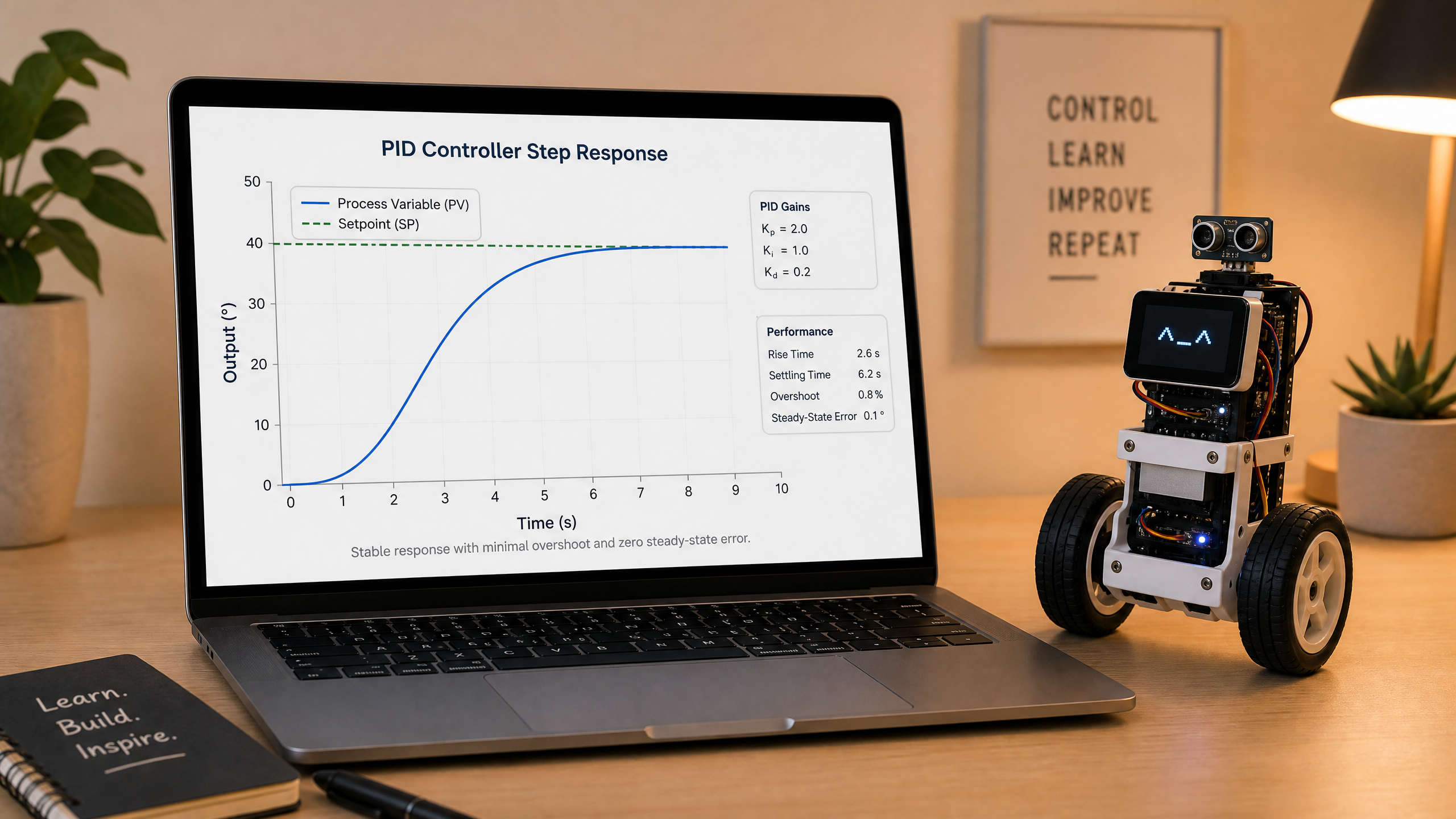
Tuning is the art of finding the right Kp, Ki, Kd values. It helps to keep in mind what each gain does for you — and how it misbehaves when pushed too far:

Gain	What it does	Too high → failure mode
Kp	Reacts to the current error; bigger error, bigger push	Oscillation; leaves steady-state error
Ki	Sums past error to erase the leftover offset	Overshoot and slow, sluggish oscillation (windup)
Kd	Reacts to the rate of change; damps the approach	Amplifies sensor noise; jittery output

A systematic approach:

1. Start with Ki = 0, Kd = 0
2. Increase Kp until the system oscillates
3. Reduce Kp to about half the oscillation value
4. Increase Ki slowly until steady-state error is eliminated
5. Add Kd if you need to reduce overshoot

This is a manual (heuristic) tuning process — the kind that works well in practice for hobby robots. There’s also a more formal recipe called the Ziegler–Nichols method: you raise Kp (with Ki = Kd = 0) until the system oscillates steadily, record that “ultimate gain” Ku and the oscillation period Tu, then plug them into fixed formulas — for a classic PID, Kp = 0.6·Ku, Ki = 1.2·Ku/Tu, Kd = 0.075·Ku·Tu. Ziegler–Nichols gives a quick starting point but tends to be aggressive (lots of overshoot), so for most hobby robotics, manual tuning by feel works fine.