SLAM: Building a Map While You Navigate

Drop a robot into a building it has never seen and ask it to make a map. It immediately hits a frustrating paradox: to know where to place a wall on the map, it needs to know where it is; but to know where it is, it needs a map to compare against. SLAM — Simultaneous Localization and Mapping — is the clever solution to this chicken-and-egg problem.

The Chicken-and-Egg Problem

Localization and mapping each assume the other is already solved:

• To build a map, you need to know the robot’s exact position when each sensor reading arrives, so you can place that reading correctly.
• To localize, you need a map to compare the current sensor reading against.

SLAM’s insight is in its first word: Simultaneously. Instead of solving one then the other, it estimates the map and the robot’s trajectory together, refining both as new data arrives. Each new laser scan slightly improves the map, and the improved map slightly improves the position estimate, and around it goes.

Front-End vs Back-End

Most SLAM systems split into two cooperating halves:

• The front-end handles perception. Its main job is scan matching — lining up the latest LiDAR scan against the previous one (or against the partial map) to estimate how far the robot moved. It may also do feature extraction, pulling out distinctive landmarks like corners. The front-end is fast but accumulates small errors over time, a problem called drift.
• The back-end handles optimization. It treats the robot’s path as a pose graph: nodes are robot positions, and edges are the measured movements between them. When errors creep in, the back-end runs pose-graph optimization to nudge all the poses into the most globally consistent arrangement.

Loop Closure: Fixing Drift

The most important trick the back-end performs is loop closure. As the robot drives, the front-end’s small errors stack up, so by the time it returns to a place it visited an hour ago, the map says it’s somewhere slightly different. Loop closure happens when the system recognizes it has returned to a previously mapped spot. It adds a new edge to the pose graph linking “now” to “back then,” and the optimizer redistributes all the accumulated drift around the whole loop. The result is a snapping-into-place effect where the map suddenly becomes consistent. Without loop closure, long corridors and large buildings come out bent and doubled.

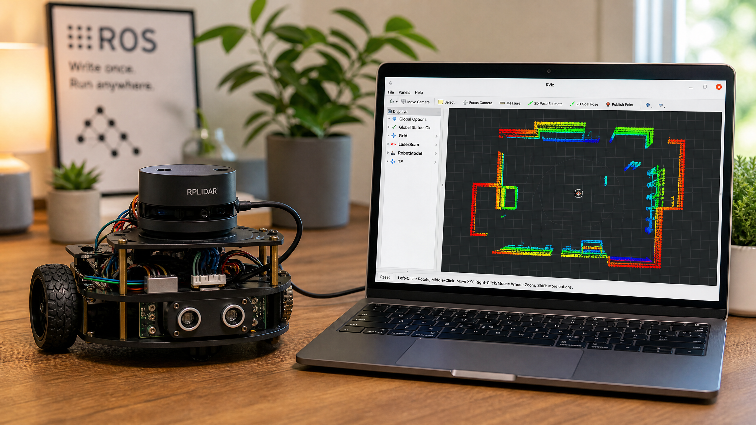
Occupancy Grid Maps

The output of most 2D SLAM systems is an occupancy grid map: a grid where each cell holds the probability that it’s occupied. Cells end up as free (drivable), occupied (a wall or obstacle), or unknown (never observed). This is exactly the map format Nav2 consumes for navigation, which is why SLAM and navigation go hand in hand.

Common 2D Approaches

• slam_toolbox: the modern default on ROS2. It’s actively maintained, supports both live mapping and refining saved maps, and handles loop closure well. This is what you should reach for today.
• gmapping: the classic particle-filter SLAM that dominated ROS1. You’ll see it referenced in older tutorials, but on ROS2 it has largely been superseded by slam_toolbox.

A Practical ROS2 Walkthrough with slam_toolbox

This builds directly on the LiDAR work from Week 10 — SLAM needs a robot publishing a laser scan on /scan and a valid TF tree (at minimum odom to base_link to your laser frame). Install slam_toolbox on Humble:

sudo apt install ros-humble-slam-toolbox

With your robot (real or simulated) running and publishing /scan plus TF, start mapping in asynchronous online mode:

ros2 launch slam_toolbox online_async_launch.py

Now open RViz and add a Map display subscribed to the /map topic. Then drive the robot slowly around the space — using teleop or your controller — and watch the occupancy grid fill in live as the LiDAR sees new areas. Drive smoothly and revisit a few places so the system gets a chance to perform loop closure; jerky, fast motion is the main cause of a messy map.

When the map looks complete, save it. The map server CLI writes two files — a .pgm image and a .yaml metadata file:

ros2 run nav2_map_server map_saver_cli -f my_map

You now have my_map.pgm and my_map.yaml. That saved map is exactly what you hand to Nav2 for autonomous navigation back in Week 18 — build it once with SLAM, then localize against it forever after.

Beyond 2D: Visual and 3D SLAM

The walkthrough above is 2D LiDAR SLAM, but the same ideas scale up. RTAB-Map builds dense 3D maps from depth and RGB cameras, and ORB-SLAM does visual SLAM purely from camera imagery by tracking visual features. These are heavier to run but essential for drones, legged robots, and anything that needs a full 3D understanding of its surroundings.

With a saved map in hand, the next challenge is letting your robot talk to the world wirelessly — next week we cover wireless communication.