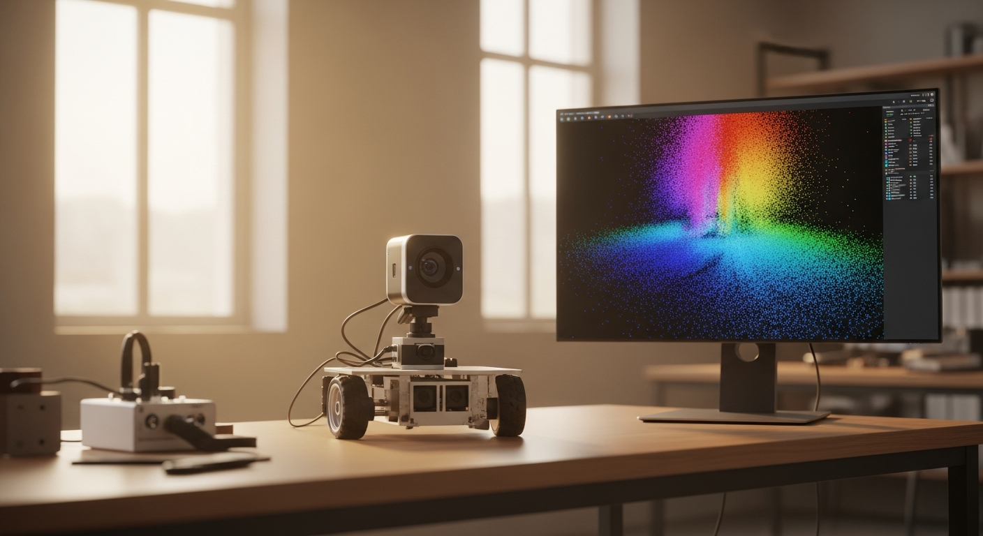
Working with Point Clouds

Back in Week 10, the RPLIDAR A1 gave your robot a 360-degree slice of the world — a flat, single-plane map of distances. That’s plenty for a wheeled robot avoiding obstacles at bumper height, but it can’t tell a low coffee table from a curb, or a low-hanging shelf from open air. To see the actual 3D shape of a scene, you need a sensor — a 3D LiDAR, a stereo pair, or a depth camera like the ones we’ll wire up in a few weeks — that returns not one flat scan, but a point cloud: tens of thousands of individual 3D points, each one a measured spot on a real surface.

This week starts a four-part block on perception, and it begins with the data structure everything else in the block builds on: how a point cloud is represented in ROS 2, how to read one in Python, and how to shrink one down to a size your code can actually keep up with.

What You’ll Learn

• What actually distinguishes a point cloud from a 2D LiDAR scan, and how ROS 2 represents one in the PointCloud2 message
• How to read point data out of a PointCloud2 in Python with sensor_msgs_py
• Why raw clouds are usually too dense to process directly, and how voxel-grid downsampling fixes that
• How to view a live point cloud in RViz2
• The pitfalls that catch beginners moving from 2D scans to 3D clouds

From a Flat Scan to a Cloud of Points

A 2D LiDAR like the RPLIDAR A1 measures distance at a set of angles, all in one horizontal plane, and publishes a sensor_msgs/msg/LaserScan — essentially a list of (angle, distance) pairs. A point cloud generalizes that idea into three dimensions: instead of one plane’s worth of distances, you get a set of full (x, y, z) coordinates, one per point the sensor detected, scattered anywhere in 3D space relative to the sensor.

ROS 2 represents this with sensor_msgs/msg/PointCloud2. Despite the name, it isn’t limited to 2D — the “2” refers to the message’s revision, not its dimensionality. A few fields matter most when you’re reading one for the first time:

Field	What it holds
height, width	Cloud shape. height == 1 means an unorganized cloud (just a flat list of points); height > 1 means an organized cloud laid out like an image grid, one point per pixel
fields	Which values each point carries — at minimum x, y, z, often also rgb or intensity
point_step	Bytes per point
row_step	Bytes per row (point_step × width)
data	The raw byte buffer holding every point, packed back to back
is_dense	False if the cloud may contain invalid (NaN) points, True if every point is guaranteed valid

That data field is just a byte blob — there’s no built-in Python list of points to loop over. That’s what the next section fixes.

Reading a Point Cloud in Python

The sensor_msgs_py package ships a point_cloud2 helper module that unpacks that raw buffer into something usable, without you touching struct offsets by hand:

import rclpy
from rclpy.node import Node
from sensor_msgs.msg import PointCloud2
from sensor_msgs_py import point_cloud2 as pc2

class CloudReader(Node):
    def __init__(self):
        super().__init__('cloud_reader')
        self.sub = self.create_subscription(
            PointCloud2, '/camera/depth/points', self.cloud_callback, 10
        )

    def cloud_callback(self, msg: PointCloud2):
        points = pc2.read_points(
            msg, field_names=('x', 'y', 'z'), skip_nans=True
        )
        count = len(points)
        if count == 0:
            self.get_logger().info('Empty cloud (skip_nans removed everything)')
            return

        # points is a structured NumPy array; access fields by name
        nearest = points['z'].min()
        self.get_logger().info(f'{count} points, nearest z: {nearest:.2f} m')

def main():
    rclpy.init()
    rclpy.spin(CloudReader())
    rclpy.shutdown()

read_points returns a structured NumPy array rather than a plain Python list, so points['x'], points['y'], and points['z'] each give you a full column of values you can run NumPy operations over directly — much faster than looping point by point in pure Python. Passing field_names=('x', 'y', 'z') skips any extra fields like rgb you don’t need yet, and skip_nans=True drops points the sensor couldn’t measure (common at a depth camera’s minimum range or on reflective surfaces), so you don’t have to filter them out yourself.

Downsampling: Making a Cloud Small Enough to Use

A single frame from a modern depth camera or 3D LiDAR can easily contain hundreds of thousands of points. Running most algorithms — obstacle detection, registration, SLAM — directly on every raw point is usually both unnecessary and too slow to keep up with a live sensor feed. The standard fix is voxel-grid downsampling: divide space into a 3D grid of small cubes (“voxels”), and collapse every point inside a voxel into a single representative point.

Open3D is the most common Python library for this kind of point cloud processing outside the ROS message layer itself:

import numpy as np
import open3d as o3d

# 'points' here is an (N, 3) NumPy array of x, y, z values,
# e.g. built from the structured array in the previous example:
# points_xyz = np.stack([points['x'], points['y'], points['z']], axis=-1)

cloud = o3d.geometry.PointCloud()
cloud.points = o3d.utility.Vector3dVector(points_xyz)

# Collapse each 2 cm cube down to one point
downsampled = cloud.voxel_down_sample(voxel_size=0.02)

print(f'{len(cloud.points)} points -> {len(downsampled.points)} points')

A larger voxel_size throws away more detail in exchange for a smaller, faster cloud; a smaller one keeps more detail at a higher point count. There’s no universally correct value — start around 1–5 cm for a tabletop-scale scene and adjust based on how much detail the task downstream actually needs.

If you’re working in C++ instead, the equivalent tool inside the ROS graph itself is the Point Cloud Library (PCL), wrapped for ROS 2 by the pcl_ros package (part of perception_pcl):

	Open3D (Python)	PCL / pcl_ros (C++)
Where it runs	Standalone script, outside the ROS message pipeline	In-graph, as ROS 2 nodes/nodelets subscribing to PointCloud2
Best for	Offline scripting, quick experiments, visualization	Production pipelines that filter/transform clouds as part of a live node graph
Install	pip install open3d	sudo apt install ros-jazzy-pcl-ros
Typical use here	voxel_down_sample(), registration, meshing	VoxelGrid, PassThrough, and other filter nodes chained in a launch file

Either tool solves the same problem; which one you reach for depends on whether you want a quick Python script or a filtering node that lives permanently in your robot’s launch file.

Visualizing a Cloud in RViz2

Before writing any processing code, it’s worth just looking at what your sensor is producing:

ros2 run rviz2 rviz2
# Add display -> By display type -> PointCloud2
# Set Topic to your cloud topic, e.g. /camera/depth/points

A few display settings are worth knowing about immediately: Size (m) controls how large each point renders (too small and a sparse cloud looks empty; too large and dense clouds turn into a solid blob), and Color Transformer lets you color points by their RGB field if the sensor provides one, or by AxisColor (coloring by height) when it doesn’t — often the fastest way to sanity-check that a cloud’s orientation and scale look right.

Common Pitfalls

Assuming PointCloud2 is 2D because of the name. The “2” is a message-format version number, left over from the original ROS 1 PointCloud message it replaced — it has nothing to do with dimensionality. Every field in a PointCloud2 is genuinely 3D.

Looping over raw bytes instead of using sensor_msgs_py. The data field is a packed byte buffer, not a Python list. Manually indexing into it with your own offset math is slow and easy to get wrong — point_cloud2.read_points() already handles the unpacking correctly.

Skipping downsampling and wondering why processing lags. A raw 300,000-point cloud run through a per-point Python loop at 10–30 Hz will fall behind almost immediately. Downsample first — even a coarse voxel grid — before running anything more expensive.

Forgetting skip_nans and getting a nan in your math. Depth sensors report a NaN point wherever they couldn’t get a valid reading. Left in, a single NaN can silently poison an average or a min/max calculation across an entire cloud. Pass skip_nans=True unless you specifically need to know which pixels were invalid.

Ignoring frame_id when combining clouds from multiple sensors. Every PointCloud2 carries a header.frame_id describing what frame its coordinates are relative to, same as any other ROS 2 message. Combining or comparing clouds from two sensors without transforming them into a common frame first — using tf2, from Week 23 — will silently misalign them even though each cloud looks fine on its own.

Recap

What you want	How to do it
Subscribe to a point cloud topic	create_subscription(PointCloud2, '<topic>', ...)
Unpack points in Python	sensor_msgs_py.point_cloud2.read_points(msg, field_names=..., skip_nans=True)
Shrink a cloud for faster processing	Voxel-grid downsampling — cloud.voxel_down_sample(voxel_size=...) in Open3D
Filter clouds inside the ROS graph (C++)	pcl_ros / perception_pcl filter nodes
View a live cloud	RViz2 → Add → PointCloud2 display, set Topic and Color Transformer
Combine clouds from multiple sensors	Transform each into a common frame with tf2 first

A point cloud is really just a big, structured list of 3D coordinates — the trick is unpacking it efficiently and cutting it down to a size your code can keep up with. Next week builds directly on that: Camera Calibration & Intrinsics, the math that lets you turn a 2D camera image into accurate 3D measurements in the first place.